Back to the Basics - Crow's Foot Diagrams

In an earlier post we touched on the topic of Entity-Relationship Diagrams (ERDs). In this post we will explain one of the more common diagramming standards for ERDs. To begin though we need to understand the types of relationships between entities.

Entity Relationships

In ERDs, entities are shown as boxes and relationships between them are shown as lines. For example, the entity Author has a relationship to the entity Book.

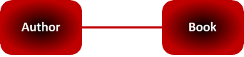
While knowing that a relationship exists between these entities is helpful, it would be more helpful to convey information about the nature of that relationship in the diagram. For instance, does every author have a relationship to a book or only some authors? Can a book exist without an author? Can a single author write multiple books? Can a book be written by multiple authors?

These relationship questions boil down to two that apply to every entity relationship:

1. Is the relationship optional or mandatory?
2. Is a single relationship or multiple relationships possible per instance of each entity?

The first question deals with the minimum number of connections (0 if optional, 1 if mandatory) and the second question deals with the maximum number of connections (1 or many). We don't try to specify a firm maximum number because whether it's 2 or 2 million, the impact on the database  design will be the same.

Many relationship diagramming methods exist for ERDs but I have found the Crow's Foot design the easiest for me to understand and the most commonly used in the companies I've worked with.

Crow's Foot Diagrams

The Crow's Foot connector uses 3 symbols to describe the minimum and maximum number of relationships:  0, 1 and < (for "many" -- I think of it as a greater-than sign)

Two symbols are used at the end of each line. The first is the minimum and the second is the maximum. There are four acceptable combinations of values as shown below.

Because the "many" symbol resembles a crow's foot, hence the name of this diagramming method.

Some people view the number zero as a letter "O" which stands for "Optional." Both interpretations are equivalent.

Now we can modify the relationship diagram for Authors and Books.

We can read the relationships in both directions. The symbol at the destination end of the line is the one that applies to that direction. These connectors show that each author writes one to many books and each book is written by one to many authors.

Note that these relationships are mandatory (i.e. minimum of one). If an author has not written any books, they cannot be considered an author. Similarly a book cannot exist without an author.

Note that the greater-than sign always means "many" even if it appears backwards (like a less-than sign).

Here is a finance example from a General Ledger data model.

In this system, financial accounts can have sub-accounts but they are not mandatory. For example, the account Office Supplies Expense may have sub-accounts called Copier Paper, Copier Toner and General Office Supplies. However the account Electricity Utility Expense has no sub-accounts because there isn't any further cost breakdown possible. This diagram reads that each account can have zero to many sub-accounts, but that each sub-account must belong to one and only one account. While sub-accounts are optional, once one is created then it has a mandatory relationship back to a single account. Sub-accounts cannot be orphans.

Next example: users and software licences.

Each user must have one and only one licence. (We will stick to the legal options only -- no pirated software!) If a person does not have a licence then they cannot be considered a user of that software. However a licence may be purchased and not assigned to any user. It may be waiting for a new hire who starts next quarter. Therefore a licence can be assigned to zero or one user.

You can begin to see that the definition of the entity can affect the definition of the relationship. The entity User contains an inherent assumption that must be understood in order for the relationship to be modeled correctly, specifically that there is no pirated software allowed.

The importance of entity definition shows up in this example as well. Here a customer buys one to many products, while a product may be bought by no one or many customers. If a person doesn't buy any of our products, they cannot be considered our customer. If however we want to track everyone who walks into our store, then we need a different model. Some people could walk in, look around and leave without buying and therefore without becoming customers. If we call everyone who enters our store "Shoppers" then that model would look like the following:

 Now the connector from Shopper to Product becomes optional.

But What About Other Combinations?

You may have noticed that selecting two values (min, max) from three different symbols (0, 1, <) should give us more than just four combinations. Obviously the maximum cannot be less than the minimum so those situations are nonsensical. However, there still are two other combinations:

• Zero and only Zero -- this effectively means there is no relationship between these two entities and therefore no line, so it is a non-existent situation in an ERD.
• Many to Many -- this means the minimum is greater than one. This situation sounds plausible.

In fact, it's not hard to imagine an entity relationship where the minimum is 2. Consider the diagram below for a genealogy database:

Each parent can have one to many children, but each child must have 2 and only 2 parents. (We'll stick to genetic parents for simplicity.) What Crow's Foot symbol should we use for representing a "2-and-only 2" relationship?

Whenever you encounter a situation like this, it means you need to redefine your entity definitions. You need to take the model to a lower level of detail.

In this case, we need to ask why we created an entity called Parent. Why not two entities called Father and Mother? Or Man and Woman? In genealogy software, those distinctions are bound to be important for reporting.

Once we create two entities out of the Parent entity (Father and Mother), the relationship to Child simplifies to a minimum value of one. Now our "2-and-only-2" relationship has been resolved.

It's important to know that relational databases cannot resolve a connection where the minimum value is greater than 1. Whenever that shows up in your model, you have to create additional entities to simplify the relationships so the minimum connector is either 0 or 1.

Short-Form Description of Entity Relationships

One more important point. When describing an entity relationship in words, the practice is to summarize it by focusing on the maximum connector values only. Minimum values are omitted for simplicity as they have less effect on the data architecture design.

For example, we would say the entity Author has a many-to-many relationship with Book.

Account has a one-to-many relationship with Sub-account, and Sub-account has a many-to-one relationship with Account.

 User has a one-to-one relationship with Licence.

While these little Crow's Foot symbols may seem insignificant, ERDs are incredibly helpful in understanding an organization's data and the business definition assumptions inherent in it. We will explore some applications of ERDs using Crow's Foot notation in future posts.

Back to the Basics - ROLAP vs MOLAP

This is part of a series of posts on some of the basic concepts of data management and business intelligence concepts. We've previously discussed the differences between OLAP and OLTP. In this post we look at the two main implementations of OLAP: Relational OLAP and Multi-dimensional OLAP.

Review of OLAP

On-Line Analytical Processing (OLAP) is a method of structuring data to permit quick aggregation queries. It makes use of the Star Schema to limit the number of query joins when connecting different data entities. Business Intelligence tools that make use of OLAP typically permit data to be arranged in rows, columns and pages, with the intersecting cells storing the aggregation results (like Excel Pivot Tables). These tools also allow interactive "drag and drop" functionality to move or add entities on rows to columns and have the aggregation results recalculate automatically.

The user experience for OLAP is similar regardless of the back-end OLAP implementation, but it is important to understand that there are two ways to store and access data in OLAP. The choice affects performance and scalability as the data mart grows and expands and it can affect which tools can be used on the front end.

Relational OLAP

Relational OLAP (ROLAP) uses standard relational databases and tables to store and deliver the data to the BI tool. However, instead of organizing the data in Third Normal Form (3NF) it is organized using a Star Schema. Any BI tool accessing a ROLAP database must be able to aggregate the cell intersection values on the fly.

Because ROLAP uses a standard relational database, the OLAP queries are written using standard SQL scripts. No special query language or functions are required.

Multi-dimensional OLAP

Multi-dimensional OLAP (MOLAP) uses a unique type of database to store and deliver the data to the BI tool. It does not consist of data tables per se but rather a multi-dimensional array that is designed to quickly aggregate the cell intersection values automatically.

Because MOLAP does not use a standard relational database, the OLAP queries are typically not written in SQL. Microsoft created a MOLAP query language for their own cube database (SSAS) called MDX and most other data cube vendors have since adopted it. (Oracle is the exception as they still use SQL with their cubes.) However MDX is not an industry standard. Microsoft owns it and they can modify it however and whenever they like.

MDX has some similarities to SQL but it is different enough that it requires dedicated training and practice. It is a very syntactic, meaning it's if you're missing a comma in a particular place it will cause the query to fail!

Comparison of ROLAP and MOLAP

Both ROLAP and MOLAP deliver all of the OLAP functionality to the end users, so from the users' perspective there is no apparent difference. There are differences in terms of performance though as well as in back-end maintenance considerations.

I have worked with multiple ROLAP and MOLAP clients across multiple database vendors and multiple BI tools. From this experience, these are the main differences I have witnessed.

Back-End Maintenance: Advantage MOLAP

MOLAP cubes can be implemented with relatively less back-end IT support than a ROLAP solution. While both require IT support, a ROLAP environment typically requires a small ETL department to maintain and load the data into the growing number of tables that support it. MOLAP also requires data loading and maintenance at the back-end, but it's usually possible for one DBA to maintain a series of MOLAP cubes.

For example, Prophix budgeting software, which sits on top of SSAS MOLAP cubes, actually permits the admin end users to do most of the data loading and maintenance processes themselves, thereby (almost) eliminating the need for IT support. I never seen this kind of functionality built on top of a ROLAP database.

Scalability: Advantage ROLAP

As a data mart grows in terms of number of fact records and number of entity members, both MOLAP and ROLAP performance can deteriorate. However, MOLAP seems to do worse when dimensions get large. While you can throw more hardware (memory and processors) at a MOLAP problem to improve performance on a large cube, it has a limited affect. Eventually the only option left is to split a MOLAP cube into smaller cubes, and that may not suit the business' analytical needs.

When ROLAP databases slow down, there is the added flexibility of being able to add more aggregate tables to the database. Aggregate tables calculate and store the sums of certain cell intersections so the BI tool doesn't have to make those calculations on the fly. This reduces the load on the BI tool and common reports that reference this aggregate table will generally load faster. These aggregate tables must be updated during the nightly ETL (Extract, Transform and Load) processes so the trade-off is a larger, slower and more complex ETL code. It also creates a more complex data model, as each BI report that is running slow may require its own new aggregate table in the background. If end users have direct access to query the data tables, these aggregate tables can make their queries more complex to build and if the aggregate tables include filter conditions, it can allow users to generate erroneous results if they are not aware of those hidden filters. While there are obviously trade-offs when considering aggregate tables, at least ROLAP provides the flexibility to choose between those trade-offs. MOLAP provides not such option.

When it comes to large-scale enterprise-wide data warehouses, MOLAP cannot keep up with the increasing data demands. ROLAP is the most common choice for these situations.

Query Language: Advantage ROLAP

ROLAP uses SQL to query the data while MOLAP uses MDX. This is a huge advantage for ROLAP for two reasons:

1. There are far more SQL developers in the world than MDX developers, so staffing your OLAP team is much easier.
2. SQL is a simpler language to learn than MDX as MDX is more syntactic than SQL. (Translation: MDX is a fussier language that is more difficult to debug!)

Summary

Each method has its own strengths and weaknesses. MOLAP is more common among small and mid-size companies while ROLAP is more common in large companies. The key is to understand your priorities and choose accordingly.

Back to the Basics - Snowflake Schema

In the last post we introduced the Star Schema. Next we will look at a modification of the Star Schema called the Snowflake Schema and explain why you should try to avoid it.

Snowflake Schema

The Star Schema is a de-normalized data structure designed to optimize aggregation query response times. It contains a fact table surrounded by a number of entity tables.

A common expansion of the Star Schema is the Snowflake.  A Snowflake Schema is simply a Star Schema where one or more of the entities have been partially normalized. This means some of the repeated details for an entity table have been hived off into a separate details table to reduce data repetition in the main entity table. An example of a Snowflake Schema is below.

Note that the original Star Schema tables are still there, but new Entity Details tables have been added around the edges, making it roughly resemble a snowflake.

Snowflake Schemas are rarely symmetric. Some entities may have multiple detail tables (such as Entity 1 above with 3) while other entities may have none (Entity 2).

What type of data is stored in the Entity Detail tables? Anything that is repeated frequently in the main Entity tables. Hierarchy levels or long textual description fields are common candidates for snowflaking.

For example, an Entity called Cost Center may have a hierarchy starting at the top with Company, then going down to Business Unit, Department and Cost Center. The facts are stored at the cost center level, so the Company, Business Unit and Department values will be repeated frequently in the entity table. Therefore, those details could be put in a separate entity details table called Cost Center Hierarchy with the cost center key remaining in the main entity table.

Avoid Snowflaking

Now that we've reviewed what the Snowflake Schema is, this is why you should avoid using it: Snowflaking works against the sole purpose of the Star Schema.

By normalizing an intentionally de-normalized data structure, the additional joins slow query response time in order to save a bit of disk space. This is ridiculous when the only reason the Star Schema exists is to improve query response time. Most instances where I have seen snowflaking used in real-world data models has been the result of a DBA (database administrator) returning to old habits and normalizing tables because that's what they've always done in the world of OLTP. It's a tough habit to break.

One Exception: Bridge Tables

A situation that diagrammatically resembles a Snowflake Schema is a Bridge Table, although I do not consider it snowflaking. A bridge table contains the conversion mapping logic between two related entity tables.

Consider two data marts, each with their own star schema. One mart contains sales data and the other manufacturing data. We want to connect the two fact tables through the Region entities to permit analysis of sales and production data together. One way to accomplish this is to conform the Region dimensions so sales and manufacturing use the same regional boundaries. That would permit a single entity table to be used by both fact tables. However, that is not always possible from a business perspective. Sales divides geography based on the number of customers and prospects in an area while manufacturing divides geography based on factory and warehouse locations. Forcing sales to use manufacturing's boundaries or vice-versa would create a lot of unnecessary hassles for the business with essentially no real benefits.

An alternative is to use a Bridge Table that equates sales regions and production regions. For example, Toronto may be in sales region Central East but in production region Ontario. The diagram below shows the Regions Bridge Table linking these two data marts.

Again, this appears similar to a snowflake of the Regions entities, but it actually involves no normalization so I don't consider it snowflaking.

A different definition of a Bridge Table exists that states they resolve many-to-many relationships between entities, but those situations should typically be resolved through the fact table. Bridge Tables should resolve different aggregation standards for similar entities. In addition to different geographical entities (described above), time is another frequent candidate for bridging when different data marts require different fiscal reporting periods.

Outrigger Tables

One other term that deserves comment comes from Ralph Kimball, one of the grandfathers of data warehousing and star schemas. While he strongly advises against snowflaking, he does permit some normalization of the star schema using something he calls Outrigger Tables. I will let him define it from his website:

"A dimension can contain a reference to another dimension table. For instance, a bank account dimension can reference a separate dimension representing the date the account was opened. These secondary dimension references are called outrigger dimensions. Outrigger dimensions are permissible, but should be used sparingly. In most cases, the correlations between dimensions should be demoted to a fact table, where both dimensions are represented as separate foreign keys."

One of Ralph's colleagues, Margy Ross, elaborates further:

"Outriggers are similar to snowflakes in that they’re used for many-to-one relationships, however they’re more limited. Outriggers are dimension tables joined to other dimension tables, but they’re just one more layer removed from the fact table, rather than being fully normalized snowflakes. Outriggers are most frequently used when one standard dimension table is referenced in another dimension, such as a hire date attribute in the employee dimension table."

Margy continues:

"Like many things in life, outriggers are acceptable in moderation, but they should be viewed as the exception rather than the rule. If outriggers are rampant in your dimensional model, it’s time to return to the drawing board given the potentially negative impact on ease-of-use and query performance."

While I agree with Margy that outriggers should be used sparingly, I fail to see a distinction between snowflaked tables and outriggers. The only apparent difference is that if snowflaked tables are small, then we can call them "outriggers" and they become permissible. I don't see the need for such a distinction. Snowflakes are snowflakes, even though they come in different sizes.

Avoid snowflaking at all costs. If there are too many outriggers or bridges in your model, it usually means the fact table is the problem and it needs to be split into two (or more) fact tables. Further discussion about cube design will follow in a later post.

Back to the Basics - Star Schema

In the last article we covered OLAP and OLTP. This article looks at the data models that support those two data structures.

Entity-Relationship Diagrams

In the mid-1970's as normalized relational databases became popular, the Entity-Relationship Diagram (ERD) emerged as a method to model and understand them. Any relational database can be modeled using an ERD, even if it is not in Third Normal Form.

The most common form of ERD's contain boxes which represent tables and lines connecting them which represent joins between foreign keys. Within the boxes all of the fields are listed, with the key fields being listed first.

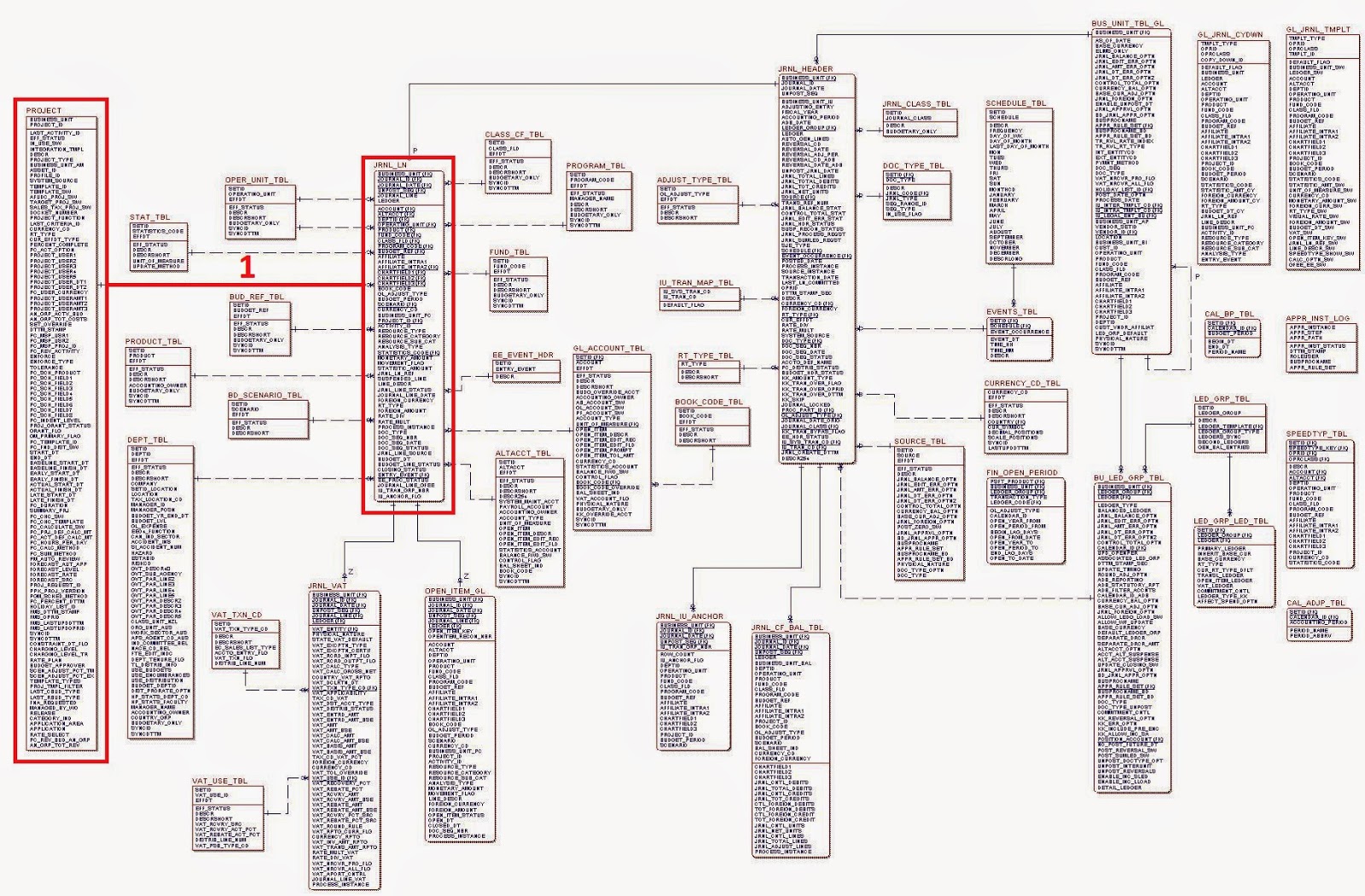
Here is an example of an ERD for one portion of a financial system database involving journal entries. It is only one of hundreds of such diagrams that together describe all of the tables in this financial database, but it serves as a good example for our purposes. It is far too small to be legible, but it is easy to see that there are a lot of tables (boxes) and a lot of joins (lines) between them.

Analytical Weaknesses of 3NF

The diagram above makes it apparent how Third Normal Form complicates database querying. Whenever a query involves a join, the query will take longer to process. The more joins in a query the slower it runs. If you have a business question that involves linking two fields from two different tables, the query performance will depend on where those two fields are located.

For example, if the two fields are in two adjacent tables, there will only be one join necessary and the query should run quickly. The diagram below highlights a query that links the Project table to the Journal Line table.

If however the two fields happen to be in the Project table and the Ledger Group table, the query will require 5 joins. The latter query will take noticeably longer to run than the first query, even though both may be valid business questions to ask of the data.

Of course, queries can have far more than 5 joins. If we consider the other 100 such ERD's in this financial system, some business questions may occasionally require fields from different modules that involve a dozen or more joins.

This inconsistent analysis query performance in 3NF caused enough of a problem that an alternative data structure was created. Enter the Star Schema.

Star Schema

Whereas 3NF treats all tables as entities, Star Schema involves two different types of tables: fact tables and entity tables.

Fact tables contain records with numeric values, such as financial transactions, and foreign keys to the entities. Fact records typically are summed but occasionally they can be counted instead.

Entity tables contain descriptive data about the facts, such as department name or product details. They permit the "slicing and dicing" of the fact records.

Combined, the fact table and entity tables make up the Star Schema.

The advantage of the Star Schema is that no matter which entities you wish to query, it involves a maximum of 2 joins. In addition, any join between entities must pass through the fact table. This guarantees there will be data to aggregate for any inter-entity query.

What is not apparent from this diagram is that it is not normalized. For example, if Entity 1 contains department data, the fields may Company, Business Unit, Department and Cost Centre. While any cost centre may only appear once in this entity table, the Company, Business Unit and Department names may repeat thousands of times. This is acceptable in Star Schema as it permits faster queries and users are not updating the records. Star Schema databases are typically updated nightly using automated processes, so repeating a business unit name thousands of times is not a problem.

Isn't denormalized data inherently inefficient though? Why not try to normalize those entity tables? That's the next topic.

Back to the Basics - OLAP vs OLTP

In the last article we looked at Third Normal Form. In this article we look at a de-normalized data structure for Business Intelligence data analysis called OLAP.

OLAP vs. OLTP

In the 1980's a new method of structuring data for analysis emerged called On-Line Analytical Processing (OLAP). It was in contrast to the prevailing method for structuring data, which was On-Line Transactional Processing (OLTP).

OLTP was designed to accomplish certain purposes with regard to databases, namely:

• efficient data storage
• fast performance when writing data (either creating or updating records)
• rapid query response time for returning individual records

OLTP accomplishes these purposes by strictly adhering to Third Normal Form (3NF). No data element is stored twice anywhere in the database, which ensures efficient storage and writing performance.

The majority of database systems in the world are OLTP. Think of your bank's system that tracks your chequing account transactions or your grocery store's Point-of-Sale system at the check-out counter that tallies your scanned products. Transactions still rule the world and OLTP systems will always have a prominent place in it.

However, for all its strengths, OLTP has a major weakness -- it can be slow when trying to aggregate large amounts of transaction data. For instance, my bank system is very fast at processing a cash withdrawal at an ATM or showing my last 10 transactions for the month. However, if an analyst at the bank wants to know the average deposit amount across all personal chequing accounts in eastern Canada in 2014, that may take a while. In fact, it may slow down the entire system while the query crunches through the millions of records necessary to find the answer.

This is why OLAP was created. It had one purpose only:

• fast performance for aggregation queries

Note there is nothing mentioned about efficient data storage or data writing performance. OLAP only cares about data aggregation performance. That single purpose is tremendously freeing because all other concerns become secondary. If storing the same data element in 3 places in the database will improve aggregation query performance, then we can do it. If it slows down data update performance, that's OK. If finding an individual record takes longer than in an OLTP system, who cares?

The main consequence of OLAP's singular purpose is that it does NOT follow 3NF. OLAP is a non-normalized data structure. Some Database Administrators (DBA's) are so used to using 3NF that they try to force normalization into OLAP, but that defeats the purpose of OLAP. Normalization slows queries because it introduces additional table joins, and joins are the enemy of fast query performance.

In the next article we will compare the data models that support OLTP and OLAP.

Back to the Basics - Third Normal Form

This is the last in a series of articles on data normalization. Click here for the previous article on Second Normal Form.

Third Normal Form

The best-known form of data normalization is Third Normal Form (3NF). When a database is said to be normalized, it usually means it's in 3NF.

Using the example from the previous article, we had our list of Employee of the Year award winners in 2NF. However, it is not in 3NF yet. In order to achieve that level of normalization, every attribute must describe the key.

 

In this case, the compound key is Year and Winner. The attributes are Reason and Department.

The Reason attribute is describing the keys. Why did the award go to Annette in 2011? Because she implemented the ERP system on time and on budget.

However, does Department actually describe the key? Is IT describing the award that went to Annette in 2011? It's really describing Annette more than the award. This means the table is not in 3NF.

Does it matter that this data is not in 3NF? It does. When we try to ask a question of the data like, "Tell me which department each winner is from," there is a challenge when we reach George Smith. He appears twice and so does him department. When they are the same, it doesn't matter which department value we return, but what if they differ? What if Department equals Sales for the 2010 record but Merchandising for the 2014 record? Which Department is correct for George? Did he change departments between those dates? Or is one of the entries simply an error? How do we know which record is wrong and which is correct? If we need to update George's department, how many records do we need to update? This kind of query ambiguity is why 3NF is important.

To resolve this problem, we need to normalize the data structure. Since Department describes the employees and not the awards, we need to create a separate table for employees as below.

Now the Employee table has a key called Employee and the Department attribute describes the key. Both tables are now compliant with 3NF.

In honour of the creator of Third Normal Form, it can be summarized in one sentence, often referred to as the Database Administrator's Oath:

Each attribute will provide a fact about the key, the whole key, and nothing but the key, so help me Codd!

Benefits of Using 3NF

Note that George is listed twice in the Award table because he won two awards, but he is listed once in the Employee table. There is no longer any ambiguity about his department. It is stored once, so queries will always return the correct department for him and any changes to his department will only have to be written in one place. To repeat from our first article, the main benefits of using normalized data structures are as follows:

• minimizing data storage
• reducing data write times
• ensuring data consistency
• ensuring data queries would return meaningful results

Sometimes the purpose of our database varies from these goals though. What is data storage costs are cheap and we no longer care about reducing write times because we rarely update a record once it is written in the database? This is where de-normalized data structures come into play. We will look at one such example in the next article.

Back to the Basics - Second Normal Form

This is the second article on normalized data structures. Click here to read about First Normal Form.

Second Normal Form

Second Normal Form (2NF) can only exist if a dataset complies with 1NF and each record has a unique compound key. A compound key uses more than one field to uniquely identify a record.

The dataset above requires two fields to unique identify each row: Year and Winner. Therefore this table is compliant with 2NF.

If a table does not have a compound key, then 2NF is automatically equivalent to 1NF.

Because 1NF and 2NF do not provide much value in a querying environment, they are rarely discussed in the real world. Either a table is 3NF compliant or it is not normalized at all.

However, the prevalence of spreadsheets means many datasets are created with a completely free data structure. Data can be organized in a spreadsheet without regard to any database rules, and as long as the data stays in a spreadsheet this isn't a problem. The challenges comes when spreadsheet data needs to be loaded into a database system or data warehouse -- that's when the need for structured data becomes apparent.

Back to the Basics - First Normal Form

Sometimes it's good to go back to the basics for a refresher lesson. Last year I did some training with analysts and realized not everyone who works with data knows what data normalization actually means. Most have heard of it but not all understand it.
So I'm going to take a few posts and go back to the basics.

Data Normalization

The concept of data normalization was first described by Edgar F. Codd in 1971 while he was working at IBM. He is credited with creating the theoretical basis for relational databases.
The purpose of normalized data structures included:

• minimizing data storage
• reducing data write times
• ensuring data consistency
• ensuring data queries would return meaningful results

The first 3 bullets can be accomplished by ensuring each data element is only stored once.  The fourth bullet requires some additional structure. All four purposes were accomplished by the normalization rules that E.F. Codd developed.

First Normal Form

There are different definitions of the first normal form (1NF) on the internet, but I find it easiest to think of it in these terms:

• Each field has only one value
• Each row has a unique key

The dataset below shows the winners of the company's Employee of the Year award for the past few years. It violates 1NF because it contains two year values in the first row. It appears that George won the award in 2010 and again in 2014, so that information has been stored in a single record.

 By separating out the 2010 and 2014 information into distinct rows, this dataset becomes compliant with 1NF. The Year column provides a unique key for each row.

However, let's take the dataset back one year when there was an unusual situation.  Two people, Sam and Maria, shared the award in 2009. Once again our dataset violates 1NF because two fields have multiple values, Winner and Department.

We solve the problem just like we did before by separating out the 2009 record into two rows, one for each award recipient. However, now the Year is no longer a unique key.  The year 2009 shows up twice, so we need to add another field to uniquely identify each row. Winner works nicely, so now Year and Winner together become the unique key. Whenever there is more than one field in a key, it is called a Compound Key, and that leads nicely into the next article on Second Normal Form (2NF).